Exploratory Data Analysis
Data Wrangling and Data Exploration
Introduction
The first two datasets used in this project are both from World Health Organization. They contains information about cases of Tuberculosis for different countries including the new cases, previous cases, drug resistant cases, total population, etc. The third dataset is from The World Bank Group which lists the GDP per capita of countries for different years in US dollars. This data is interesting because I am currently in a reserach stream at UT trying to identify potential drugs to treat tuberculosis.
The first two datasets include information about the resistance of Mycobacterium tuberculosis to drugs. Tuberculosis is linked with poverty which is why the GDP per capita was also considered. Expectations include that as the number of TB (tuberculosis) cases increase, the number of drug resistant multidrug resistant (MDR) and extensively drug resistant (XDR) TB cases will also increase. Furthermore, as GDP per capita increases, TB cases (and mortality) per 100,000 individuals should decrease since it is assumed that there is more access to healthcare and resources for treatment and prevention.
Find data:
Tidying:
join1 <- left_join(data1a, data1b, by = c("country", "year"))
head(join1)
## country region year new.pul.TB prev.treated.pul.TB prev.unk.pul.TB
## 1 Afghanistan EMR 2017 19354 2233 125
## 2 Afghanistan EMR 2018 20485 1712 NA
## 3 Albania EUR 2017 195 15 0
## 4 Albania EUR 2018 198 10 0
## 5 Algeria AFR 2017 6278 419 0
## 6 Algeria AFR 2018 6137 362 21
## new.MDR prev.MDR MDR.tested XDR pop.number TB.100k TB.num TB_mort.100k
## 1 NA NA NA 5 36296113 189 69000 30.00
## 2 NA 10 10 8 37171921 189 70000 29.00
## 3 0 0 0 0 2884169 20 580 0.34
## 4 1 1 NA NA 2882740 18 510 0.34
## 5 11 28 39 4 41389189 70 29000 7.70
## 6 2 5 7 4 42228408 69 29000 7.70
## TB_mort.num
## 1 11000
## 2 11000
## 3 10
## 4 10
## 5 3200
## 6 3300First, a left join was used to join the first two tuberculosis data sets since dataset 1a included information for 2017 and 2018 while dataset 1b contains data for many years (2000-2018). A left join was used compared to a full_join or right_join because there would be many rows with NAs (rows with year 2000-2016).
data2pivot <- data2 %>% pivot_longer(cols = c(3:4), names_to = "year",
    values_to = "GDP") %>% separate(col = "year", into = c(NA,
    "year"), sep = 1) %>% mutate(year = as.numeric(year))
head(data2pivot)
## # A tibble: 6 x 4
## country Country.Code year GDP
## <fct> <fct> <dbl> <dbl>
## 1 Aruba ABW 2017 25630.
## 2 Aruba ABW 2018 NA
## 3 Afghanistan AFG 2017 556.
## 4 Afghanistan AFG 2018 521.
## 5 Angola AGO 2017 4096.
## 6 Angola AGO 2018 3432.Then, to make it easier to join the first two datasets with the third dataset, pivot longer was used on the GDP data (dataset 2). This is due to the fact that while year is a column name in dataset 1a and 1b, for dataset 2, the GDP has two columns: 2017 and 2018. Additionally, when imported, the header of the GDP data inserted an X before the year value. This was removed using the seperate function. Mutate was then used on ‘year’ because its type was character which is incompatible with year in the tuberculosis (1a and 1b) dataset which is a numeric type (cannot be used to join).
Joining/Merging
nrow(join1)## [1] 432nrow(data2pivot)## [1] 528# Joining of all three datasets and deleting rows with NAs
join2 <- inner_join(join1, data2pivot, by = c("country", "year"))
nrow(join1) - nrow(join2)## [1] 72nrow(data2pivot) - nrow(join2)## [1] 168join2 <- join2 %>% na.omit()
nrow(join2)## [1] 222# document the type of join that you do
# (left/right/inner/full), including how many cases in each
# dataset were dropped and why you chose this particular joinInitially, the tuberculosis dataset had 432 cases while the GDP dataset had 528 cases. An inner join was chosen so that all countries remaining would contain information for tuberculosis and their GDP. This resulted in 360 observations remaining with 72 cases being dropped from the tuberculosis dataset and 168 cases dropped from the GDP dataset. Problems include that rows with NAs are more likely to be smaller and poorer countries with less documentation of the data which may skew the results.
Wrangling: filter, select, arrange, group_by, mutate, summarize
# Determining the quantile of GDP and population for each
# country
ntile <- join2 %>% mutate(ntileGDP = ntile(n = 5, x = GDP)) %>%
    mutate(ntilepop = ntile(n = 5, x = pop.number))

# Mean and standard deviation of numeric variables (excluding
# year)
join2 %>% select_if(is.numeric) %>% select(-year) %>% summarize_all(.funs = mean)
## new.pul.TB prev.treated.pul.TB prev.unk.pul.TB new.MDR prev.MDR MDR.tested
## 1 16571.29 2829.351 138.8468 135.6441 197.5495 290.7928
## XDR pop.number TB.100k TB.num TB_mort.100k TB_mort.num GDP
## 1 38.74324 33335846 98.5732 56241.17 16.46901 8344.464 14741.78join2 %>% select_if(is.numeric) %>% select(-year) %>% summarize_all(.funs = sd)## new.pul.TB prev.treated.pul.TB prev.unk.pul.TB new.MDR prev.MDR MDR.tested
## 1 84215.1 18464.84 1363.483 667.0942 1133.7 1601.977
## XDR pop.number TB.100k TB.num TB_mort.100k TB_mort.num GDP
## 1 261.0853 131603854 135.356 276737.8 32.3854 44225.92 18664.98join2 %>% summarize_all(.funs = n_distinct)## country region year new.pul.TB prev.treated.pul.TB prev.unk.pul.TB new.MDR
## 1 130 6 2 205 148 44 77
## prev.MDR MDR.tested XDR pop.number TB.100k TB.num TB_mort.100k TB_mort.num
## 1 77 86 43 222 152 142 139 132
## Country.Code GDP
## 1 130 222# top 10 Observations for extensively drug resistant TB cases
# for 2017 and 2018
ntile %>% arrange(desc(XDR)) %>% head(10)## country region year new.pul.TB prev.treated.pul.TB
## 1 Russian Federation EUR 2017 32978 26058
## 2 Ukraine EUR 2017 12840 7212
## 3 Ukraine EUR 2018 12931 6774
## 4 India SEA 2018 825939 208197
## 5 India SEA 2017 868769 176450
## 6 Belarus EUR 2017 1690 700
## 7 Tajikistan EUR 2017 2432 652
## 8 Belarus EUR 2018 1529 612
## 9 Pakistan EMR 2017 128806 15241
## 10 Peru AMR 2018 17387 3075
## prev.unk.pul.TB new.MDR prev.MDR MDR.tested XDR pop.number TB.100k TB.num
## 1 0 8206 14611 20477 3562 145530082 59 85000
## 2 0 2594 2414 5008 1001 44487709 84 37000
## 3 0 2755 2299 5054 972 44246156 80 36000
## 4 0 3232 5182 6832 493 1352642280 199 2690000
## 5 0 2152 5357 6787 466 1338676785 204 2740000
## 6 0 629 459 1088 343 9450231 37 3500
## 7 0 413 133 508 279 8880268 85 7500
## 8 0 559 425 984 185 9452617 31 2900
## 9 116 535 2102 2600 123 207906209 267 554000
## 10 0 1198 481 758 91 31989260 123 39000
## TB_mort.100k TB_mort.num Country.Code GDP ntileGDP ntilepop
## 1 8.1 12000 RUS 10750.5871 4 5
## 2 14.0 6400 UKR 2640.6757 2 5
## 3 13.0 5700 UKR 3095.1736 2 5
## 4 33.0 449000 IND 2015.5905 2 5
## 5 34.0 454000 IND 1981.4990 2 5
## 6 6.0 560 BLR 5761.7471 3 3
## 7 9.2 820 TJK 806.0416 1 3
## 8 5.9 560 BLR 6289.9386 3 3
## 9 21.0 45000 PAK 1466.8431 1 5
## 10 8.3 2700 PER 6947.2566 3 5# new variable created using mutate; proportion of XDR/MDR:
# richest countries as well as the poorest countries have the
# lowest mean percentage of MDR TB cases developing into XDR
# cases
ntile %>% mutate(perc.XDR.MDR = XDR/MDR.tested) %>% group_by(ntileGDP) %>%
summarize(mean(perc.XDR.MDR, na.rm = T))## # A tibble: 5 x 2
## ntileGDP `mean(perc.XDR.MDR, na.rm = T)`
## <int> <dbl>
## 1 1 0.0709
## 2 2 0.169
## 3 3 0.150
## 4 4 0.129
## 5 5 0.0803# Group by quantile of GDP per capita ; mean TB per 100,000
# people and mortality due to TB per 100,00 people appears to
# decrease as the percentile of GDP per capita increases
ntile %>% group_by(ntileGDP) %>% summarize(mean(TB.100k), mean(TB_mort.100k))## # A tibble: 5 x 3
## ntileGDP `mean(TB.100k)` `mean(TB_mort.100k)`
## <int> <dbl> <dbl>
## 1 1 220 49.0
## 2 2 163 19.4
## 3 3 64.0 9.93
## 4 4 29.0 2.61
## 5 5 14.9 0.811# Group by region in world: AFR=Africa; AMR=Americas;
# EMR=Eastern Mediterranean; EUR=Europe; SEAR=South-East
# Asia; WPR=Western Pacific
join2 %>% group_by(region) %>% select_if(is.numeric) %>% select(-year) %>%
summarize(mean(TB.100k), mean(TB_mort.100k))## # A tibble: 6 x 3
## region `mean(TB.100k)` `mean(TB_mort.100k)`
## <fct> <dbl> <dbl>
## 1 AFR 210 53.0
## 2 AMR 30.7 3.79
## 3 EMR 76.6 10.2
## 4 EUR 22.8 2.09
## 5 SEA 198. 26.4
## 6 WPR 153. 11.5# Maximum TB cases per 100,000 people
ntile %>% filter(TB.100k == max(TB.100k))## country region year new.pul.TB prev.treated.pul.TB prev.unk.pul.TB new.MDR
## 1 Lesotho AFR 2018 3595 728 0 51
## prev.MDR MDR.tested XDR pop.number TB.100k TB.num TB_mort.100k TB_mort.num
## 1 5 5 0 2108328 611 13000 200 4200
## Country.Code GDP ntileGDP ntilepop
## 1 LSO 1324.283 1 2# Minimum TB cases per 100,000 people
ntile %>% filter(TB.100k == min(TB.100k))## country region year new.pul.TB prev.treated.pul.TB prev.unk.pul.TB new.MDR
## 1 Barbados AMR 2017 0 0 0 0
## 2 San Marino EUR 2017 0 0 0 0
## prev.MDR MDR.tested XDR pop.number TB.100k TB.num TB_mort.100k TB_mort.num
## 1 0 0 0 286232 0 0 0.9 3
## 2 0 0 0 33671 0 0 0.0 0
## Country.Code GDP ntileGDP ntilepop
## 1 BRB 16327.61 4 1
## 2 SMR 48494.55 5 1# Group by two variables: percentile of population and year
ntile %>% group_by(ntilepop, year) %>% summarize(mean(TB.100k),
mean(TB_mort.100k))## # A tibble: 10 x 4
## # Groups: ntilepop [5]
## ntilepop year `mean(TB.100k)` `mean(TB_mort.100k)`
## <int> <dbl> <dbl> <dbl>
## 1 1 2017 89.1 9.21
## 2 1 2018 91.8 10.4
## 3 2 2017 117. 24.1
## 4 2 2018 154. 31.6
## 5 3 2017 23.3 2.31
## 6 3 2018 20.9 1.93
## 7 4 2017 106. 22.6
## 8 4 2018 147. 33.8
## 9 5 2017 124. 15.1
## 10 5 2018 124. 16.4Since most of the variables are numeric, the quantiles of GDP and the population were found and were used later to group the data. The mean and standard deviation were found for the numeric variables using the summarize_all function. Using arrange, the country that has the most extensively drug resistant TB cases for either 2017 or 2018 is the Russia followed by Ukraine and India. Using mutate to create a new variable, the proportion of of XDR/MDR appears to decrease towards the extremes of GDP per capita. Grouping by quantile of GDP per capita, mean TB cases and mortality due to TB per 100,00 people appears to decrease as the quantile of GDP per capita increases. Grouping by region, AFR has the highest mean TB cases and mortality per 100,000 people of the regions while EUR has the lowest averages.
The country with the maximum TB per 100,000 people is Lesotho in AFR and in the 1st quantile of GDP (low). The countries with the minimum TB per 100,000 people are Barbados and San Marino which both have small populations (1st quantile) and relatively high GDP. Grouping by two variables (population and year), countries in the 2nd and 4th quantile of population saw the greatest change in mean TB cases per 100,000 with both reporting an increase from 2017 to 2018. Countries in the 2nd and 4th quantile of the population also had the greatest mean mortality due to TB cases per 100,000 (as well as the greatest change between 2017 and 2018). Interestingly, the countries in the 3rd quantile had the lowest mean TB cases and mortality per 100,000 (for both 2017 and 2018).
# Correlation matrix
join2 %>% select_if(is.numeric) %>% cor() %>% round(2)
## year new.pul.TB prev.treated.pul.TB prev.unk.pul.TB
## year 1.00 0.00 0.01 0.06
## new.pul.TB 0.00 1.00 0.97 0.17
## prev.treated.pul.TB 0.01 0.97 1.00 0.06
## prev.unk.pul.TB 0.06 0.17 0.06 1.00
## new.MDR -0.03 0.39 0.47 0.02
## prev.MDR -0.06 0.47 0.53 0.08
## MDR.tested -0.05 0.43 0.49 0.07
## XDR -0.06 0.18 0.26 0.01
## pop.number 0.00 0.99 0.98 0.14
## TB.100k 0.04 0.19 0.13 0.11
## TB.num 0.00 0.99 0.96 0.21
## TB_mort.100k 0.05 0.11 0.08 0.04
## TB_mort.num 0.01 0.99 0.97 0.15
## GDP 0.01 -0.13 -0.10 -0.02
## new.MDR prev.MDR MDR.tested XDR pop.number TB.100k TB.num
## year -0.03 -0.06 -0.05 -0.06 0.00 0.04 0.00
## new.pul.TB 0.39 0.47 0.43 0.18 0.99 0.19 0.99
## prev.treated.pul.TB 0.47 0.53 0.49 0.26 0.98 0.13 0.96
## prev.unk.pul.TB 0.02 0.08 0.07 0.01 0.14 0.11 0.21
## new.MDR 1.00 0.96 0.98 0.96 0.43 0.04 0.38
## prev.MDR 0.96 1.00 0.99 0.93 0.51 0.06 0.47
## MDR.tested 0.98 0.99 1.00 0.96 0.47 0.05 0.42
## XDR 0.96 0.93 0.96 1.00 0.23 0.00 0.17
## pop.number 0.43 0.51 0.47 0.23 1.00 0.13 0.98
## TB.100k 0.04 0.06 0.05 0.00 0.13 1.00 0.23
## TB.num 0.38 0.47 0.42 0.17 0.98 0.23 1.00
## TB_mort.100k 0.01 0.03 0.02 -0.01 0.07 0.86 0.13
## TB_mort.num 0.38 0.46 0.42 0.17 0.98 0.21 0.98
## GDP -0.09 -0.08 -0.09 -0.06 -0.10 -0.40 -0.13
## TB_mort.100k TB_mort.num GDP
## year 0.05 0.01 0.01
## new.pul.TB 0.11 0.99 -0.13
## prev.treated.pul.TB 0.08 0.97 -0.10
## prev.unk.pul.TB 0.04 0.15 -0.02
## new.MDR 0.01 0.38 -0.09
## prev.MDR 0.03 0.46 -0.08
## MDR.tested 0.02 0.42 -0.09
## XDR -0.01 0.17 -0.06
## pop.number 0.07 0.98 -0.10
## TB.100k 0.86 0.21 -0.40
## TB.num 0.13 0.98 -0.13
## TB_mort.100k 1.00 0.16 -0.32
## TB_mort.num 0.16 1.00 -0.13
## GDP -0.32 -0.13 1.00The correlation matrix shows that the strongest positive correlations are between new pulmonary TB cases and population number; new pulmonary TB cases and total number of TB cases; new pulmonary TB cases and total mortality due to TB; previous MDR TB cases and number of MDR cases that were tested for additional resistance. The strongest negative correlations are GDP and the TB cases per 100,000 people; GDP and TB mortality per 100,000 people.
Visualizing
# GGPlot 1: Scatterplot
ntile %>% ggplot(aes(x = TB.100k, y = TB_mort.100k)) + geom_point(aes(color = ntileGDP)) +
ggtitle("TB Cases and Mortality") + xlab("TB Cases per 100,000 people") +
ylab("TB mortality per 100,000 people") + scale_fill_brewer() +
scale_y_continuous(breaks = c(25, 50, 75, 100, 125, 150,
175, 200)) + scale_x_continuous(breaks = c(100, 200,
300, 400, 500, 600)) + labs(color = "GDP") + theme_classic()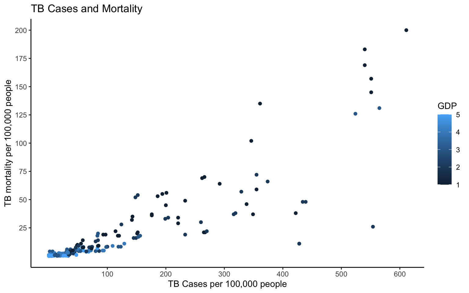 This graph shows that as TB cases increase, TB mortality also increases per 100,000 people. Contrastingly, TB cases and mortality have a negative relationship with GDP per capita. This suggests that countries with lower GDP have higher occurrences of TB and mortality due to TB which is expected since there is less funding towards preventative measures as well as resources and access to treatment.
# GGPlot 2: Boxplot
ntile %>% ggplot(aes(group = region, x = region, y = TB.100k)) +
geom_boxplot() + geom_jitter(alpha = 0.3, aes(color = ntilepop,
size = ntilepop)) + ggtitle("TB cases for each Region") +
xlab("Region") + ylab("TB Cases per 100,000 people") + labs(color = "Population",
size = "Population") + theme_light()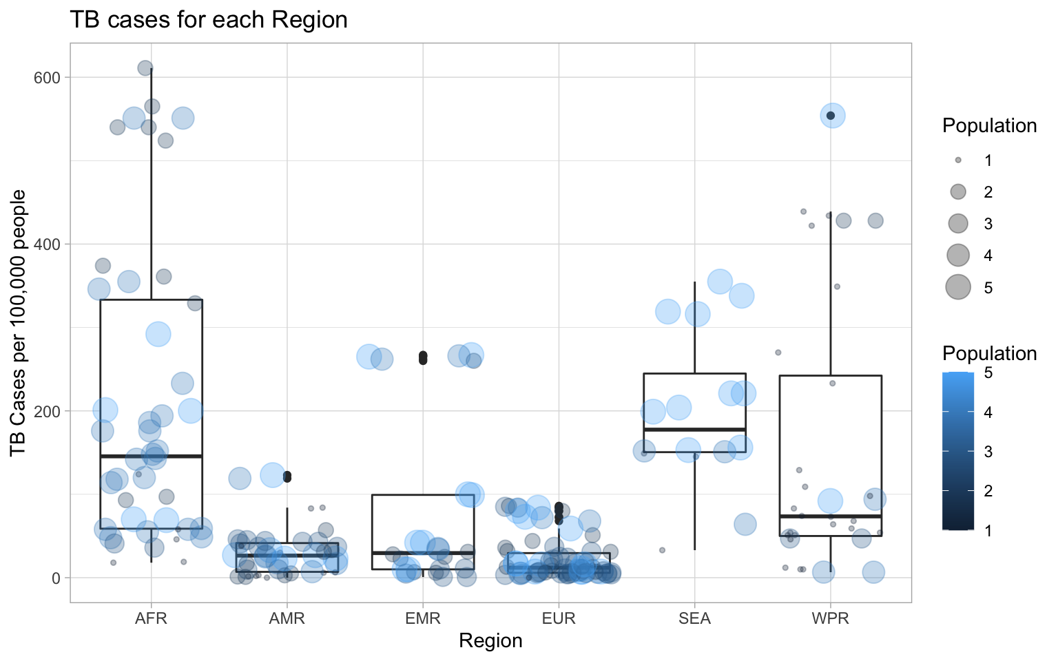 The boxplot shows that the median of TB cases for 100,000 people is highest in SEA. Previously, summary statistics showed that AFR had the highest mean. From the boxplot, it is clear that the distribution is skewed resulting in a higher median than mean. The spread is largest for AFR as well. The countries in AMR, EMR, and EUR all have relatively low median values. When grouped by region, there is not an obvious relationship between the population and TB cases per 100,000 people.
# GGPlot 3: Stacked Bar plot
ntile$year <- factor(ntile$year, levels = c("2017", "2018"))
ggplot(ntile, aes(x = ntileGDP, y = TB_mort.100k, fill = year)) +
geom_bar(stat = "summary", fun.y = "mean", position = "dodge") +
geom_errorbar(stat = "summary", position = "dodge") + xlab("Quantile of GDP per capita") +
ylab("TB Mortality per 100,000 people") + ggtitle("GDP per Capita and TB mortality per 100,000 people") +
theme_grey() + scale_y_continuous(breaks = c(10, 20, 30,
40, 50, 60))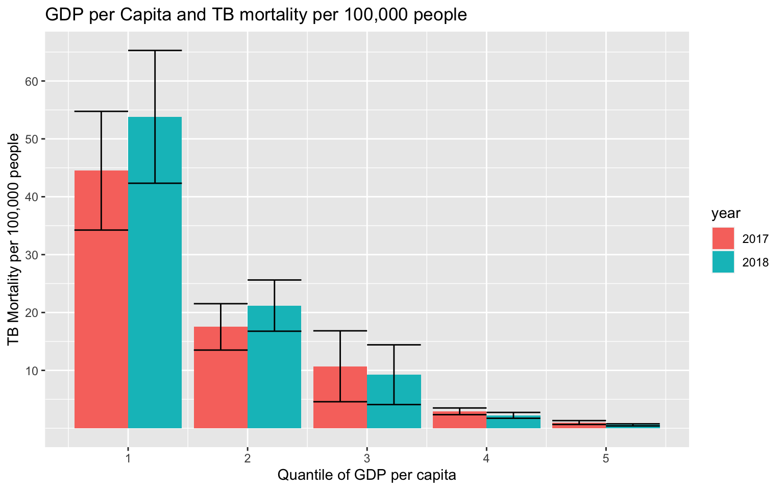 A stacked bar plot was used to demonstrate how increasing GDP per capita results in a lower TB mortality on average. The biggest change in TB mortality between 2017 and 2018 is represented in the countries in the 1st quantile of GDP per capita (however, the error bars are overlapping). As the quantile of GDP increases, the spread of the data (error bars) also decrease.
Dimensionality Reduction
# Prepare data by scaling
joinPCA <- join2 %>% select_if(is.numeric) %>% scale %>% na.omit
join_pca <- princomp(joinPCA)
summary(join_pca, loadings = T)
## Importance of components:
## Comp.1 Comp.2 Comp.3 Comp.4 Comp.5
## Standard deviation 2.5078967 1.6468586 1.4044384 1.01775753 0.96840866
## Proportion of Variance 0.4512861 0.1946011 0.1415266 0.07432267 0.06728992
## Cumulative Proportion 0.4512861 0.6458872 0.7874138 0.86173646 0.92902637
## Comp.6 Comp.7 Comp.8 Comp.9
## Standard deviation 0.86661846 0.371251458 0.202421301 0.145441708
## Proportion of Variance 0.05388756 0.009889379 0.002939985 0.001517786
## Cumulative Proportion 0.98291394 0.992803315 0.995743300 0.997261086
## Comp.10 Comp.11 Comp.12 Comp.13
## Standard deviation 0.127383707 0.1098210941 0.0756806126 0.052799805
## Proportion of Variance 0.001164288 0.0008653747 0.0004109623 0.000200031
## Cumulative Proportion 0.998425374 0.9992907485 0.9997017107 0.999901742
## Comp.14
## Standard deviation 3.700566e-02
## Proportion of Variance 9.825826e-05
## Cumulative Proportion 1.000000e+00
##
## Loadings:
## Comp.1 Comp.2 Comp.3 Comp.4 Comp.5 Comp.6 Comp.7 Comp.8
## year 0.729 0.674
## new.pul.TB -0.356 0.246 -0.118 0.147
## prev.treated.pul.TB -0.362 0.188 -0.138 -0.465
## prev.unk.pul.TB 0.656 -0.728 0.101
## new.MDR -0.297 -0.385 -0.616
## prev.MDR -0.320 -0.344 0.524
## MDR.tested -0.310 -0.372 0.177
## XDR -0.235 -0.474 0.124
## pop.number -0.361 0.210 -0.147
## TB.100k 0.213 0.602 -0.241 0.708
## TB.num -0.354 0.253 -0.100 0.131 0.239
## TB_mort.100k 0.192 0.602 -0.358 -0.670
## TB_mort.num -0.354 0.255 -0.101 -0.115
## GDP -0.404 0.157 -0.890
## Comp.9 Comp.10 Comp.11 Comp.12 Comp.13 Comp.14
## year
## new.pul.TB -0.304 0.175 -0.790 -0.156
## prev.treated.pul.TB 0.688 -0.130 0.264 -0.111
## prev.unk.pul.TB
## new.MDR -0.402 -0.197 -0.295 -0.212 0.203
## prev.MDR 0.382 -0.267 -0.185 -0.219 -0.151 0.416
## MDR.tested -0.102 0.177 -0.821
## XDR 0.537 0.512 0.332 0.201
## pop.number -0.139 -0.605 0.616 0.164
## TB.100k
## TB.num -0.307 0.115 -0.437 0.509 0.358 0.199
## TB_mort.100k
## TB_mort.num 0.424 -0.667 0.390
## GDP# Choose number of PC to keep convert standard deviations to
# eigenvalues
eigval <- join_pca$sdev^2
# proportion of variance explained by each PC
varprop = round(eigval/sum(eigval), 2)
ggplot() + geom_bar(aes(y = varprop, x = 1:14), stat = "identity") +
xlab("") + geom_path(aes(y = varprop, x = 1:14)) + geom_text(aes(x = 1:14,
y = varprop, label = round(varprop, 2)), vjust = 1, col = "white",
size = 5) + scale_y_continuous(breaks = seq(0, 0.6, 0.2),
labels = scales::percent) + scale_x_continuous(breaks = 1:14)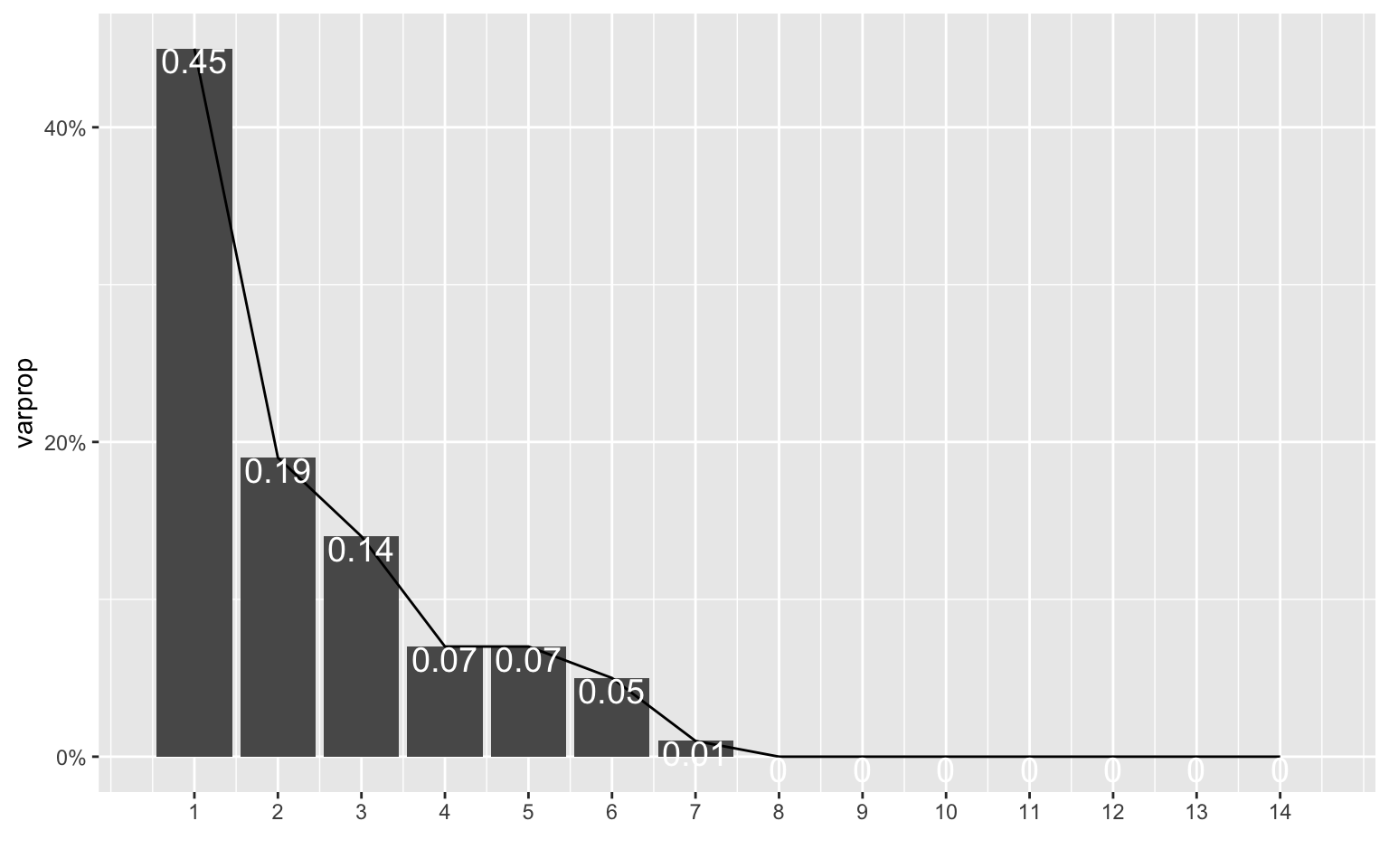
# Plot for PCA (PC1 and PC2)
join2 %>% na.omit %>% mutate(PC1 = join_pca$scores[, 1], PC2 = join_pca$scores[,
    2]) %>% ggplot(aes(x = PC1, y = PC2, color = region, size = GDP)) +
    geom_point() + ggtitle("PCA Plot") + theme(legend.position = "none")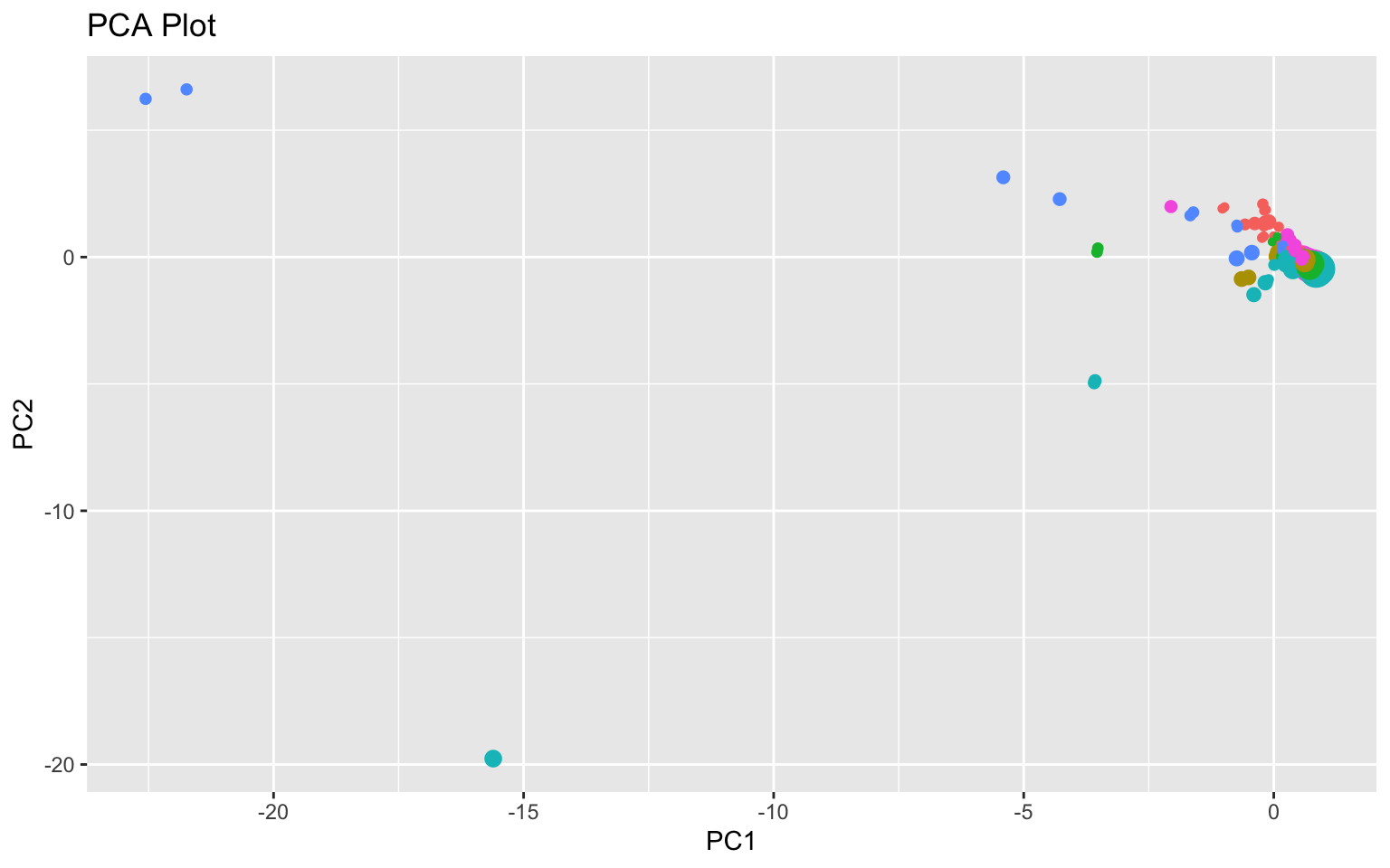
# Plot for PCA (PC3 and PC4)
join2 %>% na.omit %>% mutate(PC3 = join_pca$scores[, 3], PC4 = join_pca$scores[,
    4]) %>% ggplot(aes(x = PC3, y = PC4, color = region, size = GDP)) +
    geom_point() + ggtitle("PCA Plot") + theme(legend.position = "none")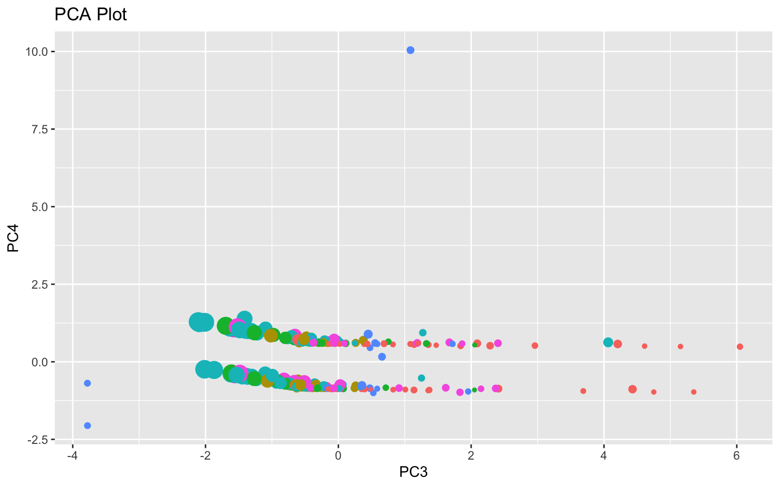
# Plot of loadings
join_pca$loadings[1:14, 1:2] %>% as.data.frame %>% rownames_to_column %>%
    ggplot() + geom_hline(aes(yintercept = 0), lty = 2) + geom_vline(aes(xintercept = 0),
    lty = 2) + ylab("PC2") + xlab("PC1") + geom_segment(aes(x = 0,
    y = 0, xend = Comp.1, yend = Comp.2), arrow = arrow(), col = "red") +
    geom_label(aes(x = Comp.1 * 1.1, y = Comp.2 * 1.1, label = rowname)) +
    ggtitle("Plot of Loadings")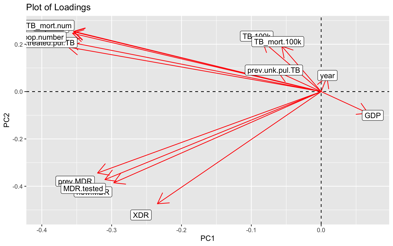
# biplot combining loadings plot and PC score plot
library("factoextra")
fviz_pca_biplot(join_pca)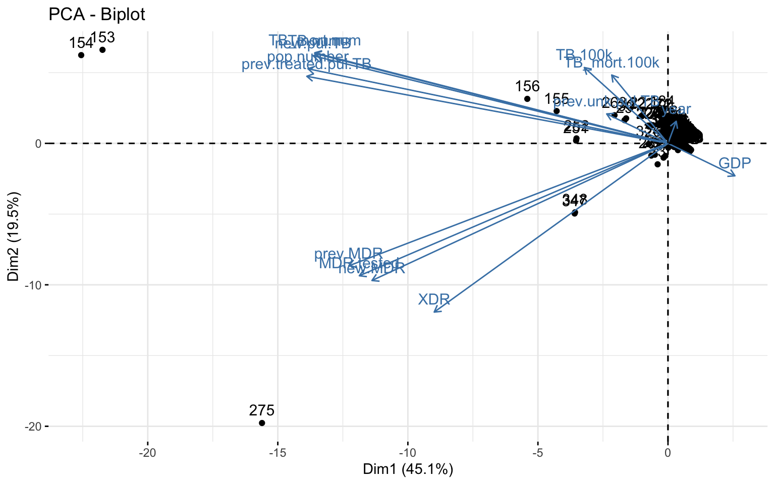
Based on the scree plot and cumulative proportion of variance (and Kaiser’s rule), 3 to 4 PCs should be chosen. High scores on PC1 indicate low TB cases (new, previous, MDR TB, mortality, etc.) and low population. For PC2, high scores indicate high TB cases and mortality per 100,000 people but lower resistant (MDR and XDR) TB cases as well as lower GDP per capita. For PC3, high scores indicate lower cases of resistant TB cases and lower TB cases and mortality per 100,000 people but higher GDP. On the PCA plot, there appears to be some seperation based on GDP looking at PC3 (larger dots on the right). Finally, high scores PC4 indicate high numbers of confirmed TB cases with unknown TB treatment history.
The plot of loadings helps visualize which variances contribute to which of the PCs with a smaller angle between vectors showing higher correlation. Therefore, GDP is negatively correlated to the other variables and mainly differs based on PC1. Contrastingly, other variables such as new cases of pulmonary TB, previous treated pulmonary TB cases, total TB cases, etc. are almost redundant.
## R version 3.6.1 (2019-07-05)
## Platform: x86_64-apple-darwin15.6.0 (64-bit)
## Running under: macOS Mojave 10.14.6
##
## Matrix products: default
## BLAS:   /Library/Frameworks/R.framework/Versions/3.6/Resources/lib/libRblas.0.dylib
## LAPACK: /Library/Frameworks/R.framework/Versions/3.6/Resources/lib/libRlapack.dylib
##
## locale:
## [1] en_US.UTF-8/en_US.UTF-8/en_US.UTF-8/C/en_US.UTF-8/en_US.UTF-8
##
## attached base packages:
## [1] stats     graphics  grDevices utils     datasets  methods   base
##
## other attached packages:
##  [1] factoextra_1.0.6 forcats_0.5.0    stringr_1.4.0    dplyr_0.8.5
##  [5] purrr_0.3.3      readr_1.3.1      tidyr_1.0.2      tibble_2.1.3
##  [9] ggplot2_3.3.0    tidyverse_1.3.0  knitr_1.28
##
## loaded via a namespace (and not attached):
##  [1] tidyselect_1.0.0 xfun_0.12        haven_2.2.0      lattice_0.20-40
##  [5] colorspace_1.4-1 vctrs_0.2.4      generics_0.0.2   htmltools_0.4.0
##  [9] yaml_2.2.1       utf8_1.1.4       rlang_0.4.5      ggpubr_0.2.5
## [13] pillar_1.4.3     withr_2.1.2      glue_1.3.2       DBI_1.1.0
## [17] dbplyr_1.4.2     modelr_0.1.6     readxl_1.3.1     lifecycle_0.2.0
## [21] ggsignif_0.6.0   munsell_0.5.0    blogdown_0.18    gtable_0.3.0
## [25] cellranger_1.1.0 rvest_0.3.5      codetools_0.2-16 evaluate_0.14
## [29] labeling_0.3     fansi_0.4.1      broom_0.5.5      Rcpp_1.0.4
## [33] formatR_1.7      backports_1.1.5  scales_1.1.0     jsonlite_1.6.1
## [37] farver_2.0.3     fs_1.3.2         hms_0.5.3        digest_0.6.25
## [41] stringi_1.4.6    ggrepel_0.8.2    bookdown_0.18    grid_3.6.1
## [45] cli_2.0.2        tools_3.6.1      magrittr_1.5     crayon_1.3.4
## [49] pkgconfig_2.0.3  ellipsis_0.3.0   xml2_1.2.5       reprex_0.3.0
## [53] lubridate_1.7.4  assertthat_0.2.1 rmarkdown_2.1    httr_1.4.1
## [57] rstudioapi_0.11  R6_2.4.1         nlme_3.1-145     compiler_3.6.1
## [1] "2020-07-24 14:53:51 CDT"## sysname
## "Darwin"
## release
## "18.7.0"
## version
## "Darwin Kernel Version 18.7.0: Tue Aug 20 16:57:14 PDT 2019; root:xnu-4903.271.2~2/RELEASE_X86_64"
## nodename
## "Cara-Yijin-Zou.local"
## machine
## "x86_64"
## login
## "yijinzou"
## user
## "yijinzou"
## effective_user
## "yijinzou"Cara Zou
Interests include dentistry and computer science.