Modeling, Testing, and Predicting
Modeling
Introduction
This dataset is comprised of a merged dataset from World Health Organization and The World Bank Group. It consists of information about cases of Tuberculosis including new pulmonary cases, previous cases, drug resistant cases (MDR and XDR), mortality due to tuberculosis, etc. This dataset also contains information about country, region, year (2017 or 2018), population number, and GDP per capita in US dollars.
MANOVA testing
 #H0: For each response variable, the means of the groups are equal
 #H1: For at least one response variable, at least one group mean differs
head(TB_Data)
## country region year new.pul.TB prev.treated.pul.TB
prev.unk.pul.TB new.MDR prev.MDR
## 1 Albania EUR 2017 195 15 0 0 0
## 2 Algeria AFR 2017 6278 419 0 11 28
## 3 Algeria AFR 2018 6137 362 21 2 5
## 4 American Samoa WPR 2017 3 0 0 1 0
## 5 Andorra EUR 2017 1 0 0 0 0
## 6 Angola AFR 2018 31098 6623 0 0 0
## MDR.tested XDR pop.number TB.100k TB.num TB_mort.100k
TB_mort.num GDP
## 1 0 0 2884169 20.0 580 0.34 10 4532.889
## 2 39 4 41389189 70.0 29000 7.70 3200 4048.285
## 3 7 4 42228408 69.0 29000 7.70 3300 4278.850
## 4 1 0 55620 10.0 6 0.85 0 11398.777
## 5 0 0 77001 1.5 1 0.12 0 39134.393
## 6 0 0 30809787 355.0 109000 72.00 22000 3432.386man1<-manova(cbind(new.pul.TB,prev.treated.pul.TB,prev.unk.pul.TB, new.MDR, prev.MDR, XDR, pop.number, TB.100k, TB_mort.100k, GDP)~region, data=TB_Data)
summary(man1)## Df Pillai approx F num Df den Df Pr(>F)
## region 5 1.2666 7.1585 50 1055 < 2.2e-16 ***
## Residuals 216
## ---
## Signif. codes: 0 '***' 0.001 '**' 0.01 '*' 0.05 '.' 0.1
' ' 1There are alot of assumptions for the MANOVA test which indicates that they are usually hard to test and/or meet. These assumptions include: random samples, independent observations, dependent variables have multivariate normality, homogeneity of within-group covariance matrices for each dependent variable and equal covariance between any two dependent variables, linear relationships amoung dependent variables, no extreme univariate or multivariate outliers, and no multicollinearity. The dataset would likely not have been able to meet the assumptions, especially since many of the variables are likely correlated (e.g.: new drug resistant TB cases is likely related to previous/new TB cases ).
For the MANOVA, only 10 dependent variables were chosen. For example, only one of TB.100k (TB cases per 100,000 people) and TB.num (TB cases total) since they are likely to be highly related. The p-value (< 2.2e-16) is significant for the MANOVA test, therefore, for at least one of the response variables, the mean between regions is different.
Univariate ANOVA testing
summary.aov(man1)## Response new.pul.TB :
## Df Sum Sq Mean Sq F value Pr(>F)
## region 5 3.7015e+11 7.4029e+10 13.356 2.385e-11 ***
## Residuals 216 1.1972e+12 5.5427e+09
## ---
## Signif. codes: 0 '***' 0.001 '**' 0.01 '*' 0.05 '.' 0.1
' ' 1
##
## Response prev.treated.pul.TB :
## Df Sum Sq Mean Sq F value Pr(>F)
## region 5 1.1311e+10 2262181943 7.6302 1.268e-06 ***
## Residuals 216 6.4039e+10 296477285
## ---
## Signif. codes: 0 '***' 0.001 '**' 0.01 '*' 0.05 '.' 0.1
' ' 1
##
## Response prev.unk.pul.TB :
## Df Sum Sq Mean Sq F value Pr(>F)
## region 5 30299516 6059903 3.4395 0.005189 **
## Residuals 216 380558289 1761844
## ---
## Signif. codes: 0 '***' 0.001 '**' 0.01 '*' 0.05 '.' 0.1
' ' 1
##
## Response new.MDR :
## Df Sum Sq Mean Sq F value Pr(>F)
## region 5 4062809 812562 1.8615 0.1023
## Residuals 216 94285428 436507
##
## Response prev.MDR :
## Df Sum Sq Mean Sq F value Pr(>F)
## region 5 12235002 2447000 1.9446 0.08818 .
## Residuals 216 271810715 1258383
## ---
## Signif. codes: 0 '***' 0.001 '**' 0.01 '*' 0.05 '.' 0.1
' ' 1
##
## Response XDR :
## Df Sum Sq Mean Sq F value Pr(>F)
## region 5 468938 93788 1.388 0.2299
## Residuals 216 14595646 67572
##
## Response pop.number :
## Df Sum Sq Mean Sq F value Pr(>F)
## region 5 7.5761e+17 1.5152e+17 10.661 3.61e-09 ***
## Residuals 216 3.0700e+18 1.4213e+16
## ---
## Signif. codes: 0 '***' 0.001 '**' 0.01 '*' 0.05 '.' 0.1
' ' 1
##
## Response TB.100k :
## Df Sum Sq Mean Sq F value Pr(>F)
## region 5 1375556 275111 22.228 < 2.2e-16 ***
## Residuals 216 2673438 12377
## ---
## Signif. codes: 0 '***' 0.001 '**' 0.01 '*' 0.05 '.' 0.1
' ' 1
##
## Response TB_mort.100k :
## Df Sum Sq Mean Sq F value Pr(>F)
## region 5 81943 16388.6 23.624 < 2.2e-16 ***
## Residuals 216 149845 693.7
## ---
## Signif. codes: 0 '***' 0.001 '**' 0.01 '*' 0.05 '.' 0.1
' ' 1
##
## Response GDP :
## Df Sum Sq Mean Sq F value Pr(>F)
## region 5 2.0424e+10 4084759281 15.597 4.243e-13 ***
## Residuals 216 5.6568e+10 261891068
## ---
## Signif. codes: 0 '***' 0.001 '**' 0.01 '*' 0.05 '.' 0.1
' ' 1Of the 10 dependent variables tested, the univariate ANOVAs with a p-value <0.05 include: new.pul.TB, prev.treated.pul.TB, prev.unk.pul.TB, pop.number, TB.100k, TB_mort.100k, and GDP.
Post hoc t-testing
# region in world: AFR=Africa; AMR=Americas;
# EMR=Eastern Mediterranean; EUR=Europe; SEAR=South-East
# Asia; WPR=Western Pacific

#New pulmonary tuberculosis cases
pairwise.t.test(TB_Data$new.pul.TB,TB_Data$region,p.adj="none")
##
## Pairwise comparisons using t tests with pooled SD
##
## data: TB_Data$new.pul.TB and TB_Data$region
##
## AFR AMR EMR EUR SEA
## AMR 0.71 - - - -
## EMR 0.83 0.60 - - -
## EUR 0.64 0.96 0.54 - -
## SEA 2.1e-11 7.2e-12 2.5e-09 3.8e-13 -
## WPR 0.80 0.92 0.67 0.87 4.7e-11
##
## P value adjustment method: none#Previously treated pulmonary tuberculosis cases
pairwise.t.test(TB_Data$prev.treated.pul.TB,TB_Data$region,p.adj="none")##
## Pairwise comparisons using t tests with pooled SD
##
## data: TB_Data$prev.treated.pul.TB and TB_Data$region
##
## AFR AMR EMR EUR SEA
## AMR 0.88 - - - -
## EMR 0.90 0.80 - - -
## EUR 0.98 0.89 0.87 - -
## SEA 1.3e-07 1.0e-07 2.4e-06 3.1e-08 -
## WPR 0.96 0.93 0.87 0.98 3.7e-07
##
## P value adjustment method: none#Confirmed pulmonary TB cases with unknown TB treatment history
pairwise.t.test(TB_Data$prev.unk.pul.TB,TB_Data$region,p.adj="none")##
## Pairwise comparisons using t tests with pooled SD
##
## data: TB_Data$prev.unk.pul.TB and TB_Data$region
##
## AFR AMR EMR EUR SEA
## AMR 0.97315 - - - -
## EMR 0.98235 0.99463 - - -
## EUR 0.74157 0.77669 0.80590 - -
## SEA 0.00023 0.00031 0.00090 0.00028 -
## WPR 0.98122 0.95689 0.96726 0.74643 0.00042
##
## P value adjustment method: none#Population Number
pairwise.t.test(TB_Data$pop.number,TB_Data$region,p.adj="none")##
## Pairwise comparisons using t tests with pooled SD
##
## data: TB_Data$pop.number and TB_Data$region
##
## AFR AMR EMR EUR SEA
## AMR 1.00 - - - -
## EMR 0.61 0.62 - - -
## EUR 0.92 0.93 0.64 - -
## SEA 5.7e-10 9.3e-10 1.2e-07 1.5e-10 -
## WPR 0.76 0.77 0.46 0.68 8.6e-10
##
## P value adjustment method: none#TB cases per 100,000 individuals
pairwise.t.test(TB_Data$TB.100k,TB_Data$region,p.adj="none")##
## Pairwise comparisons using t tests with pooled SD
##
## data: TB_Data$TB.100k and TB_Data$region
##
## AFR AMR EMR EUR SEA
## AMR 3.4e-12 - - - -
## EMR 4.2e-06 0.11090 - - -
## EUR 1.2e-15 0.72536 0.04362 - -
## SEA 0.72362 7.4e-07 0.00082 4.6e-08 -
## WPR 0.02843 6.2e-06 0.01175 1.5e-07 0.18283
##
## P value adjustment method: none#TB mortality cases per 100,000 individuals
pairwise.t.test(TB_Data$TB_mort.100k,TB_Data$region,p.adj="none")##
## Pairwise comparisons using t tests with pooled SD
##
## data: TB_Data$TB_mort.100k and TB_Data$region
##
## AFR AMR EMR EUR SEA
## AMR 2.3e-15 - - - -
## EMR 9.7e-10 0.34679 - - -
## EUR < 2e-16 0.74776 0.19773 - -
## SEA 0.00066 0.00411 0.05824 0.00109 -
## WPR 1.2e-10 0.21678 0.85228 0.09768 0.06676
##
## P value adjustment method: none#GDP
pairwise.t.test(TB_Data$GDP,TB_Data$region,p.adj="none")##
## Pairwise comparisons using t tests with pooled SD
##
## data: TB_Data$GDP and TB_Data$region
##
## AFR AMR EMR EUR SEA
## AMR 0.03154 - - - -
## EMR 0.00053 0.10499 - - -
## EUR 1.0e-13 2.1e-07 0.00652 - -
## SEA 0.82314 0.16977 0.01100 2.6e-07 -
## WPR 0.00045 0.13530 0.81059 0.00098 0.01345
##
## P value adjustment method: noneBonferroni correction
#MANOVA: 1
#ANOVA: 11
#T-tests: 15* 7= 105

#Probability of a type I error if unadjusted
1-(1-0.05)^117
## [1] 0.9975245#New alpha
0.05/(1+10+105)## [1] 0.0004310345The total number of tests conducted is 117, therefore if unadjusted, the probability of at least one type I error is 0.9975. Therefore, the bonferroni correction was used to obtain the new alpha value of 0.00043 so that the overall alpha value remains at 0.05.
Using this new alpha value, the MANOVA is still significant. The ANOVAs of new.pul.TB, prev.treated.pul.TB, pop.number, TB.100k, TB_mort.100k, and GDP are still significant. Only the ANOVA of prev.unk.pul.TB is no longer significant (p-value=0.005189). For the post-hoc analysis of the new pulmonary TB cases, previously treated pulmonary TB, and population number only the means of SEA are different from the other regions. For TB.100k there are significant differences between AFR/AMR, AFR/EMR, AFR/EUR, AMR/SEA, AMR/WPR, SEA/EMR, EUR/SEA, and EUR/WPR. For the TB mortality for every 100,000 individuals, AFR is significantly different from the other regions. For GDP, AFR/EMR, AFR/EUR, AFR/WPR, AMR/EUR, EUR/SEA, and EUR/WPR are significantly different.
Randomization test: PERMANOVA
#H0: The centroid and dispersion of points is the same for the different regions
#H1: The centroid and dispersion of points is different for at least one of the different regions


#compute distances/dissimilarities
dists<-TB_Data%>%dplyr::select(new.pul.TB,prev.treated.pul.TB,prev.unk.pul.TB, new.MDR, prev.MDR, XDR, pop.number, TB.100k, TB_mort.100k, GDP)%>%dist()


#compute observed F
SST<- sum(dists^2)/150
SSW<-TB_Data%>%group_by(region)%>%dplyr::select(new.pul.TB,prev.treated.pul.TB,prev.unk.pul.TB, new.MDR, prev.MDR, XDR, pop.number, TB.100k, TB_mort.100k, GDP)%>%
 do(d=dist(.[2:3],"euclidean"))%>%ungroup()%>%
 summarise(sum(d[[1]]^2)/50 + sum(d[[2]]^2)/50+ sum(d[[3]]^2)/50)%>%pull
F_obs<-((SST-SSW)/2)/(SSW/147) #observed F statistic
F_obs
## [1] 21739142596# compute null distribution for F
Fs<-replicate(1000,{
new<-TB_Data%>%mutate(region=sample(region)) #permute the region vector
SSW<-new%>%group_by(region)%>%dplyr::select(new.pul.TB,prev.treated.pul.TB,prev.unk.pul.TB, new.MDR, prev.MDR, XDR, pop.number, TB.100k, TB_mort.100k, GDP)%>%
do(d=dist(.[2:3],"euclidean"))%>%ungroup()%>%
summarise(sum(d[[1]]^2)/50 + sum(d[[2]]^2)/50+ sum(d[[3]]^2)/50)%>%pull
((SST-SSW)/2)/(SSW/147) #calculate new F on randomized data
})
{hist(Fs,prob = T); abline(v=F_obs, col="red", add=T)}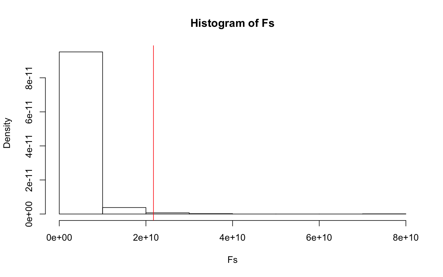
mean(Fs>F_obs) #p-value ## [1] 0.01Since the data is unlikely to meet the assumptions of the MANOVA, a randomization-test MANOVA (PERMANOVA) was conducted which resulted in a p-value < 0.05 (significant). Therefore the null hypothesis is rejected in favor of the alternative hypothesis that there is a significant difference between the centroid and/or the spread of the points is not equal between the different regions. This therefore supports the conclusion of the MANOVA conducted previously.
Linear regression model
TB_Data$GDP_c <- TB_Data$GDP - mean(TB_Data$GDP, na.rm = T)
TB_Data$TB_mort.100k_c <- TB_Data$TB_mort.100k - mean(TB_Data$TB_mort.100k, na.rm = T)
fit1<-lm(TB_mort.100k_c ~ GDP_c*region, data=TB_Data)

#uncorrected SEs
summary(fit1)
##
## Call:
## lm(formula = TB_mort.100k_c ~ GDP_c * region, data =
TB_Data)
##
## Residuals:
## Min 1Q Median 3Q Max
## -54.036 -5.622 -1.086 1.755 144.129
##
## Coefficients:
## Estimate Std. Error t value Pr(>|t|)
## (Intercept) 1.059e+00 1.514e+01 0.070 0.9443
## GDP_c -2.858e-03 1.179e-03 -2.423 0.0162 *
## regionAMR -1.472e+01 1.595e+01 -0.923 0.3572
## regionEMR -6.498e+00 1.605e+01 -0.405 0.6860
## regionEUR -1.457e+01 1.557e+01 -0.936 0.3505
## regionSEA -3.136e+01 3.331e+01 -0.942 0.3475
## regionWPR -5.678e+00 1.582e+01 -0.359 0.7200
## GDP_c:regionAMR 2.651e-03 1.328e-03 1.996 0.0472 *
## GDP_c:regionEMR 2.457e-03 1.211e-03 2.029 0.0437 *
## GDP_c:regionEUR 2.789e-03 1.188e-03 2.349 0.0198 *
## GDP_c:regionSEA -6.893e-04 2.812e-03 -0.245 0.8066
## GDP_c:regionWPR 2.541e-03 1.204e-03 2.110 0.0361 *
## ---
## Signif. codes: 0 '***' 0.001 '**' 0.01 '*' 0.05 '.' 0.1
' ' 1
##
## Residual standard error: 25.98 on 210 degrees of freedom
## Multiple R-squared: 0.3884, Adjusted R-squared: 0.3564
## F-statistic: 12.12 on 11 and 210 DF, p-value: < 2.2e-16For the model with uncorrected standard errors, controlling for region, for every increase of 1 USD of GDP from the mean, the number of cases of mortality due to tuberculosis per 100,000 people decreases by 2.858e-03. Compared to the reference region of AFR and controlling for GDP, the mean number of cases of mortality due to tuberculosis per 100,000 people decreases for all regions: AMR (1.472e+01), EMR(6.498e+00), EUR (1.457e+01), SEA (3.136e+01), and WPR (5.678e+00). The coefficient for the interactions describe the difference in the effect of GDP on the mortality due to tuberculosis per 100,00 people depending on which region the country is in (the slope difference between the regions). For example, the slope difference between AFR and: AMR (2.651e-03), EMR (2.457e-03), EUR (2.789e-03), SEA (-6.893e-04), and WPR (2.541e-03).
Plot the regression
TB_Data%>%ggplot(aes(x=GDP_c, y=TB_mort.100k_c,group=region))+geom_point(aes(color=region))+geom_smooth(method = 'lm',se=F, aes(color=region))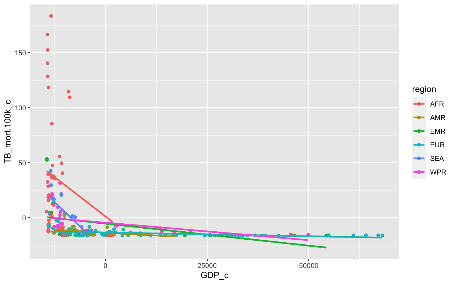
Asumptions
#Linear relationship between each predictor and response (no scatterplot for region since it is categorical)
ggplot(TB_Data, aes(x=GDP_c, y=TB_mort.100k_c,group=region))+geom_point(aes(color=region))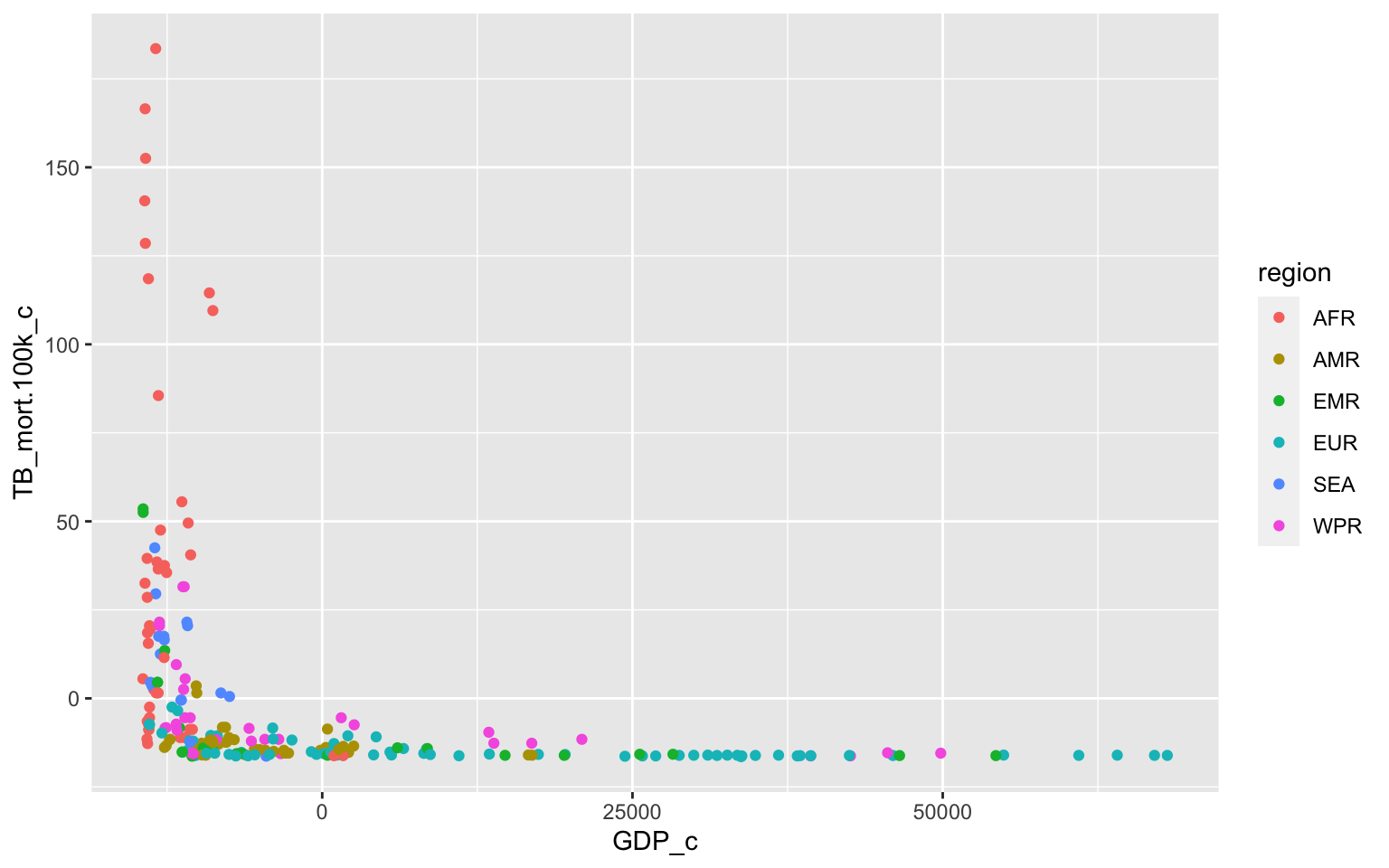
# Confirm normality of residuals
qqnorm(fit1$residuals, main = "QQ-plot of Model Residuals")
qqline(fit1$residuals, col = "red")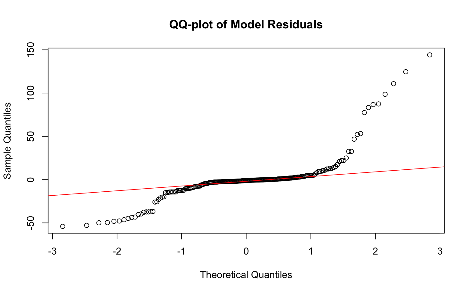
# Confirm equal variance
plot(fit1$fitted.values, fit1$residuals, xlab = "Fitted Values",
    ylab = "Residuals", pch = 20)
abline(h = 0, col = "red")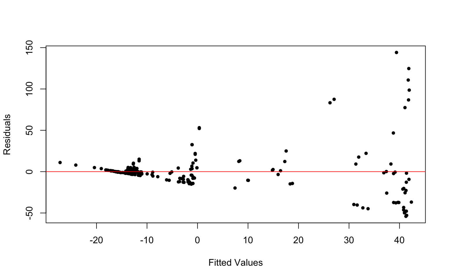
library(sandwich); library(lmtest)
bptest(fit1)
##
## studentized Breusch-Pagan test
##
## data: fit1
## BP = 58.313, df = 11, p-value = 1.905e-08The data fails all assumptions. The scatterplot does not show a linear relationship between GDP and TB_mort.100k. The QQ-plot of the model residuals is also not normal. There is also a funneling pattern in the residual plot which indicates that it does not meet the assumption of equal variance (homoskedasticity). This is again confirmed by the Breusch-Pagan test which concluded that the homoskedasticity assumption is not met (p-value=1.905e-08).
Recompute regression results with robust standard errors
#robust SEs
coeftest(fit1, vcov = vcovHC(fit1))
##
## t test of coefficients:
##
## Estimate Std. Error t value Pr(>|t|)
## (Intercept) 1.0589e+00 2.0328e+01 0.0521 0.95851
## GDP_c -2.8577e-03 1.7036e-03 -1.6775 0.09494 .
## regionAMR -1.4716e+01 2.0333e+01 -0.7238 0.47001
## regionEMR -6.4979e+00 2.0762e+01 -0.3130 0.75462
## regionEUR -1.4572e+01 2.0334e+01 -0.7166 0.47441
## regionSEA -3.1361e+01 2.2356e+01 -1.4028 0.16215
## regionWPR -5.6775e+00 2.0456e+01 -0.2776 0.78163
## GDP_c:regionAMR 2.6510e-03 1.7052e-03 1.5546 0.12155
## GDP_c:regionEMR 2.4566e-03 1.7146e-03 1.4327 0.15342
## GDP_c:regionEUR 2.7895e-03 1.7036e-03 1.6374 0.10305
## GDP_c:regionSEA -6.8927e-04 1.9443e-03 -0.3545 0.72331
## GDP_c:regionWPR 2.5408e-03 1.7056e-03 1.4897 0.13781
## ---
## Signif. codes: 0 '***' 0.001 '**' 0.01 '*' 0.05 '.' 0.1
' ' 1A model with robust standard errors should be used if the data is heteroskedastic. With uncorrected standard errors, the coefficient estimates of the main effect of GDP (p-value = 0.0162) was significant. The interactions GDP_c:regionAMR (p-value= 0.0472), GDP_c:regionEMR (p-value= 0.0437), GDP_c:regionEUR (p-value= 0.0198), and GDP_c:regionWPR (p-value= 0.0361) were also significant. Contrastingly, using the more robust SEs (more conservative), none of the coefficient estimates are still significant.
Effect Size
summary(fit1)$adj.r.squared## [1] 0.3563608The adjusted r-squared of 0.356 indicates that 35.6% of variation in the mean number of cases of mortality due to tuberculosis per 100,000 people is explained by the model.
Regression but without interactions
fit2<-lm(TB_mort.100k_c ~ GDP_c+region, data=TB_Data)
summary(fit2)
##
## Call:
## lm(formula = TB_mort.100k_c ~ GDP_c + region, data =
TB_Data)
##
## Residuals:
## Min 1Q Median 3Q Max
## -49.946 -6.211 -1.696 2.397 146.834
##
## Coefficients:
## Estimate Std. Error t value Pr(>|t|)
## (Intercept) 3.394e+01 4.177e+00 8.125 3.49e-14 ***
## GDP_c -2.055e-04 1.101e-04 -1.866 0.063421 .
## regionAMR -4.759e+01 5.783e+00 -8.230 1.80e-14 ***
## regionEMR -3.978e+01 6.834e+00 -5.822 2.10e-08 ***
## regionEUR -4.572e+01 5.796e+00 -7.888 1.53e-13 ***
## regionSEA -2.635e+01 7.646e+00 -3.446 0.000684 ***
## regionWPR -3.867e+01 6.261e+00 -6.177 3.23e-09 ***
## ---
## Signif. codes: 0 '***' 0.001 '**' 0.01 '*' 0.05 '.' 0.1
' ' 1
##
## Residual standard error: 26.19 on 215 degrees of freedom
## Multiple R-squared: 0.3638, Adjusted R-squared: 0.3461
## F-statistic: 20.49 on 6 and 215 DF, p-value: < 2.2e-16Examining only the main effects, the effect of GDP is no longer significant while all the coeficient estimates for region are now significant.
Linear regression model with bootstrapped standard errors
# repeat 5000 times, saving the coefficients each time
samp_distn<-replicate(5000, {
 boot_TB<-TB_Data[sample(nrow(TB_Data),replace=TRUE),]
 fit3<-lm(TB_mort.100k_c ~ GDP_c*region, data=boot_TB)
 coef(fit3)
})

#Estimated SEs
samp_distn%>%t%>%as.data.frame%>%summarise_all(sd)
## (Intercept) GDP_c regionAMR regionEMR regionEUR
regionSEA regionWPR GDP_c:regionAMR
## 1 38.5149 0.003056803 38.5189 38.75788 38.51718 41.48764
38.50866 0.003058287
## GDP_c:regionEMR GDP_c:regionEUR GDP_c:regionSEA
GDP_c:regionWPR
## 1 0.0030693 0.00305682 0.003327013 0.003059335Bootstrapped standard errors are used when the data is non-normal as well. Compared to the original standard errors, the standard errors for all the coefficient estimates increased (more conservative). The p-values are therefore higher as well because of the higher standard errors. Compared to the robust standard errors, the bootstrapped standard errors are also higher. Therefore, the p-values are also higher (more conservative).
Logistic regression predicting a binary categorical variable
BinaryTB<-TB_Data%>%mutate(y = as.numeric(ifelse(XDR > 0, 1, 0)))
fit4<-glm(y~region+TB.100k+pop.number,data=BinaryTB,family=binomial(link="logit"))
coeftest(fit4)
##
## z test of coefficients:
##
## Estimate Std. Error z value Pr(>|z|)
## (Intercept) -2.5554e+00 5.5591e-01 -4.5968 4.291e-06 ***
## regionAMR 2.2980e-01 6.5681e-01 0.3499 0.7264340
## regionEMR 1.2454e+00 6.4541e-01 1.9296 0.0536624 .
## regionEUR 2.2567e+00 5.6757e-01 3.9761 7.005e-05 ***
## regionSEA 4.0806e-01 8.6513e-01 0.4717 0.6371581
## regionWPR -2.4001e-01 6.4077e-01 -0.3746 0.7079782
## TB.100k 5.4362e-03 1.5506e-03 3.5059 0.0004551 ***
## pop.number 3.8675e-08 1.0182e-08 3.7984 0.0001456 ***
## ---
## Signif. codes: 0 '***' 0.001 '**' 0.01 '*' 0.05 '.' 0.1
' ' 1exp(coef(fit4))## (Intercept) regionAMR regionEMR regionEUR regionSEA
regionWPR TB.100k pop.number
## 0.07766039 1.25834993 3.47417743 9.55178621 1.50390035
0.78661626 1.00545098 1.00000004A binary variable was created that measures whether there are any XDR (extensively drug resistant tuberculosis) cases in a country. Controlling for TB.100k and population number, the odds of having a XDR TB case are 1.25 times higher for the region AMR than AFR. The odds for the other regions compared to AFR: EMR (3.47), EUR (9.55), SEA (1.50), WPR (0.79). The region with the lowest odds of a country having a case of XDR TB is WPR. The region that has the highest odds of a country having a case of XDR TB is EUR. Controlling for region and TB.100k, for every 1-unit increase in population number, odds of having a case of XDR TB change by a factor of 1.00000004. Controlling for region and population number, for every 1-unit increase in TB.100k, odds of having a case of XDR TB change by a factor of 1.00545098 (increase by 0.54%).
Confusion Matrix
prob <- predict(fit4, type = "response") #get predictions
pred <- ifelse(prob > 0.5, 1, 0)
table(truth = BinaryTB$y, prediction = pred) %>% addmargins
## prediction
## truth 0 1 Sum
## 0 109 23 132
## 1 34 56 90
## Sum 143 79 222#Classification Function
class_diag<-function(probs,truth){
tab<-table(factor(probs>.5,levels=c("FALSE","TRUE")),truth)
acc=sum(diag(tab))/sum(tab)
sens=tab[2,2]/colSums(tab)[2]
spec=tab[1,1]/colSums(tab)[1]
ppv=tab[2,2]/rowSums(tab)[2]
if(is.numeric(truth)==FALSE & is.logical(truth)==FALSE) truth<-as.numeric(truth)-1
#CALCULATE EXACT AUC
ord<-order(probs, decreasing=TRUE)
probs <- probs[ord]; truth <- truth[ord]
TPR=cumsum(truth)/max(1,sum(truth))
FPR=cumsum(!truth)/max(1,sum(!truth))
dup<-c(probs[-1]>=probs[-length(probs)], FALSE)
TPR<-c(0,TPR[!dup],1); FPR<-c(0,FPR[!dup],1)
n <- length(TPR)
auc<- sum( ((TPR[-1]+TPR[-n])/2) * (FPR[-1]-FPR[-n]) )
data.frame(acc,sens,spec,ppv,auc)
}
class_diag(prob, BinaryTB$y)## acc sens spec ppv auc
## 1 0.7432432 0.6222222 0.8257576 0.7088608 0.8367845From the confusion matrix, the model has an accuracy of 0.743 which is fair. The sensitivity or true positive rate is 0.622 which is poor. The specificity or true negative rate is 0.826 which is good. The precision or positive predictive value of the model is 0.709 which is fair.
Density of log-odds (logit)
BinaryTB$logit<-predict(fit4) #get predicted log-odds
BinaryTB$factor.y<-factor(BinaryTB$y,levels=c(1,0))
ggplot(BinaryTB,aes(logit, fill=factor.y))+geom_density(alpha=.3)+
geom_vline(xintercept=0,lty=2)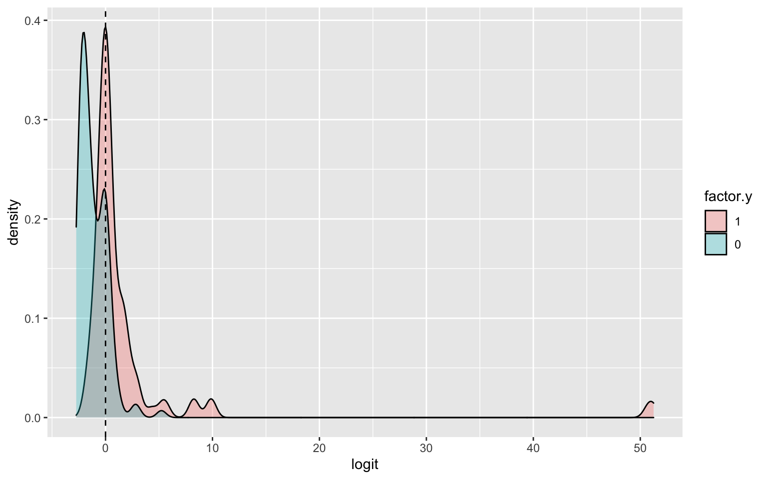 #### ROC Curve
library(plotROC)
prob <- predict(fit4, type = "response")
ROCplot1 <- ggplot(BinaryTB) + geom_roc(aes(d = y, m = prob),n.cuts = 0)+geom_segment(aes(x=0,xend=1,y=0,yend=1),lty=2)
ROCplot1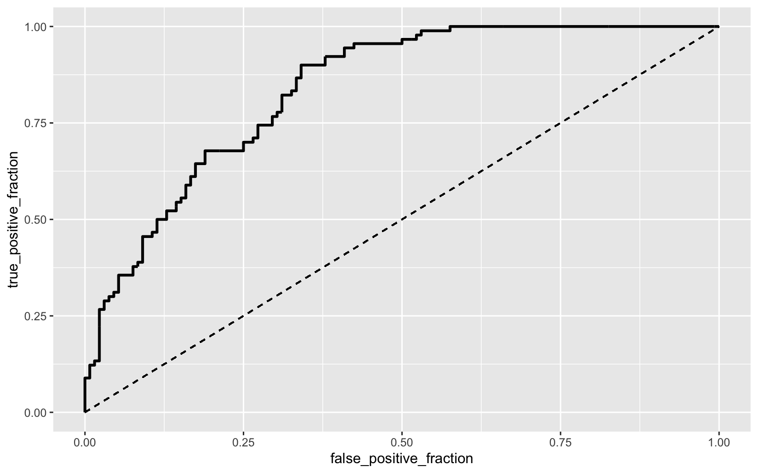
calc_auc(ROCplot1)## PANEL group AUC
## 1 1 -1 0.8367845The AUC is determined to be 0.837 which suggests that the model is good at predicting whether a country has a case of XDR TB (the probability that a randomly selected country with a case of XDR TB has a higher prediction than a randomly selected country without a case of XDR TB).
10-fold CV
k = 10
data1 <- BinaryTB[sample(nrow(BinaryTB)), ] #put dataset in random order
folds <- cut(seq(1:nrow(BinaryTB)), breaks = k, labels = F) #create folds
diags <- NULL
for (i in 1:k) {
# FOR EACH OF 10 FOLDS
train <- data1[folds != i, ] #CREATE TRAINING SET
test <- data1[folds == i, ] #CREATE TESTING SET
truth <- test$y
fit <- glm(y~region+TB.100k+pop.number,data=BinaryTB,family=binomial(link="logit"))
probs <- predict(fit, newdata = test, type = "response")
diags <- rbind(diags, class_diag(probs, truth))
}
apply(diags, 2, mean) #AVERAGE THE DIAGNOSTICS ACROSS THE 10 FOLDS
## acc sens spec ppv auc
## 0.7434783 0.6364087 0.8170467 0.7267569 0.8221299The out of sample confusion matrix for this model has: accuracy (0.742- fair), sensitivity (0.625- poor), specificity (0.811- good), precision (0.692- poor). Although, precision decreased from fair to poor, the classifications did not change greatly. The AUC also did not change significantly which suggests that there was not overfitting.
LASSO (least absolute shrinkage and selection operator) Regression
head(BinaryTB)## country region year new.pul.TB prev.treated.pul.TB
prev.unk.pul.TB new.MDR prev.MDR
## 1 Albania EUR 2017 195 15 0 0 0
## 2 Algeria AFR 2017 6278 419 0 11 28
## 3 Algeria AFR 2018 6137 362 21 2 5
## 4 American Samoa WPR 2017 3 0 0 1 0
## 5 Andorra EUR 2017 1 0 0 0 0
## 6 Angola AFR 2018 31098 6623 0 0 0
## MDR.tested XDR pop.number TB.100k TB.num TB_mort.100k
TB_mort.num GDP GDP_c
## 1 0 0 2884169 20.0 580 0.34 10 4532.889 -10208.887
## 2 39 4 41389189 70.0 29000 7.70 3200 4048.285 -10693.491
## 3 7 4 42228408 69.0 29000 7.70 3300 4278.850 -10462.926
## 4 1 0 55620 10.0 6 0.85 0 11398.777 -3342.999
## 5 0 0 77001 1.5 1 0.12 0 39134.393 24392.617
## 6 0 0 30809787 355.0 109000 72.00 22000 3432.386
-11309.391
## TB_mort.100k_c y logit factor.y
## 1 -16.129009 0 -0.07841423 0
## 2 -8.769009 1 -0.57416872 1
## 3 -8.769009 1 -0.54714847 1
## 4 -15.619009 0 -2.73891183 0
## 5 -16.349009 0 -0.28754952 0
## 6 55.530991 0 0.56598835 0LassoTB<-BinaryTB%>%dplyr::select(region,year,new.pul.TB, prev.treated.pul.TB, prev.unk.pul.TB,new.MDR, prev.MDR, MDR.tested,pop.number, TB.100k, TB.num, TB_mort.100k, TB_mort.num,GDP,y)
fit5 <- glm(y~.,data=LassoTB,family=binomial(link="logit"))
library(glmnet)
x <- model.matrix(fit5)[, -1]
y <- as.matrix(LassoTB$y)
cv <- cv.glmnet(x, y, family = "binomial")
lasso <- glmnet(x, y, family = "binomial", lambda = cv$lambda.1se)
coef(lasso)## 19 x 1 sparse Matrix of class "dgCMatrix"
## s0
## (Intercept) -1.184453e+00
## regionAMR -9.067621e-03
## regionEMR 4.794832e-01
## regionEUR 1.507004e+00
## regionSEA 3.001555e-01
## regionWPR -2.811042e-01
## year .
## new.pul.TB .
## prev.treated.pul.TB .
## prev.unk.pul.TB .
## new.MDR 6.021496e-04
## prev.MDR .
## MDR.tested .
## pop.number 6.064149e-09
## TB.100k 2.758181e-03
## TB.num .
## TB_mort.100k .
## TB_mort.num .
## GDP -1.286157e-05Variables with a non-zero coefficient from LASSO will be retained in the model: region, new.MDR, pop.number, TB.100k, and GDP. Therefore, these are the most important predictors of if a country has atleast one case of XDR TB.
Perform 10-fold CV using LASSO model
#Model with just non-zero lasso coefficient estimates
fit6 <- glm(y ~ region+new.MDR+pop.number+TB.100k+GDP, data = LassoTB, family = "binomial")

prob6 <- predict(fit6, type = "response")
class_diag(prob6, LassoTB$y)
## acc sens spec ppv auc
## 1 0.7972973 0.6333333 0.9090909 0.826087 0.8883838#10-fold CV
k = 10
data1 <- LassoTB[sample(nrow(LassoTB)), ] #put dataset in random order
folds <- cut(seq(1:nrow(LassoTB)), breaks = k, labels = F) #create folds
diags <- NULL
for (i in 1:k) {
# FOR EACH OF 10 FOLDS
train <- data1[folds != i, ] #CREATE TRAINING SET
test <- data1[folds == i, ] #CREATE TESTING SET
truth <- test$y
fit <- glm(y ~ region+new.MDR+pop.number+TB.100k+GDP, data = LassoTB, family = "binomial")
probs <- predict(fit, newdata = test, type = "response")
diags <- rbind(diags, class_diag(probs, truth))
}
apply(diags, 2, mean) #AVERAGE THE DIAGNOSTICS ACROSS THE 10 FOLDS## acc sens spec ppv auc
## 0.7976285 0.6386111 0.9093773 0.8284127 0.8826206This new model’s out of sample accuracy is 0.797 which is fair. It is slightly higher than the previous model’s out of sample accuracy which was 0.743. The AUC also slightly increased from 0.839 to 0.886 (both models are good predictors of if there are XDR TB cases in a country).
## R version 3.6.1 (2019-07-05)
## Platform: x86_64-apple-darwin15.6.0 (64-bit)
## Running under: macOS Mojave 10.14.6
##
## Matrix products: default
## BLAS:
/Library/Frameworks/R.framework/Versions/3.6/Resources/lib/libRblas.0.dylib
## LAPACK:
/Library/Frameworks/R.framework/Versions/3.6/Resources/lib/libRlapack.dylib
##
## locale:
## [1]
en_US.UTF-8/en_US.UTF-8/en_US.UTF-8/C/en_US.UTF-8/en_US.UTF-8
##
## attached base packages:
## [1] stats graphics grDevices utils datasets methods base
##
## other attached packages:
## [1] glmnet_3.0-2 Matrix_1.2-18 plotROC_2.2.1
lmtest_0.9-37 zoo_1.8-7 sandwich_2.5-1
## [7] forcats_0.5.0 stringr_1.4.0 dplyr_0.8.5 purrr_0.3.3
readr_1.3.1 tidyr_1.0.2
## [13] tibble_2.1.3 ggplot2_3.3.0 tidyverse_1.3.0
knitr_1.28
##
## loaded via a namespace (and not attached):
## [1] Rcpp_1.0.4 lubridate_1.7.4 lattice_0.20-40
foreach_1.4.8 assertthat_0.2.1
## [6] digest_0.6.25 R6_2.4.1 cellranger_1.1.0 plyr_1.8.6
backports_1.1.5
## [11] reprex_0.3.0 evaluate_0.14 httr_1.4.1 blogdown_0.18
pillar_1.4.3
## [16] rlang_0.4.5 readxl_1.3.1 rstudioapi_0.11
rmarkdown_2.1 labeling_0.3
## [21] splines_3.6.1 munsell_0.5.0 broom_0.5.5
compiler_3.6.1 modelr_0.1.6
## [26] xfun_0.12 pkgconfig_2.0.3 shape_1.4.4 mgcv_1.8-31
htmltools_0.4.0
## [31] tidyselect_1.0.0 bookdown_0.18 codetools_0.2-16
fansi_0.4.1 crayon_1.3.4
## [36] dbplyr_1.4.2 withr_2.1.2 grid_3.6.1 nlme_3.1-145
jsonlite_1.6.1
## [41] gtable_0.3.0 lifecycle_0.2.0 DBI_1.1.0 magrittr_1.5
scales_1.1.0
## [46] cli_2.0.2 stringi_1.4.6 farver_2.0.3 fs_1.3.2
xml2_1.2.5
## [51] generics_0.0.2 vctrs_0.2.4 iterators_1.0.12
tools_3.6.1 glue_1.3.2
## [56] hms_0.5.3 yaml_2.2.1 colorspace_1.4-1 rvest_0.3.5
haven_2.2.0
## [1] "2020-07-24 14:55:18 CDT"## sysname
## "Darwin"
## release
## "18.7.0"
## version
## "Darwin Kernel Version 18.7.0: Tue Aug 20 16:57:14 PDT
2019; root:xnu-4903.271.2~2/RELEASE_X86_64"
## nodename
## "Cara-Yijin-Zou.local"
## machine
## "x86_64"
## login
## "yijinzou"
## user
## "yijinzou"
## effective_user
## "yijinzou"Cara Zou
Interests include dentistry and computer science.